Inciter performance

Strong scaling

The following figures quantify strong scaling of the different solvers in Inciter (Compressible flow solver).

Strong scaling of the time stepping phase (i.e., excluding setup) running DiagCG, ALECG, and the DG single-material Euler solvers using a 794-million-cell mesh without large-file I/O up to about 50 thousand CPUs. The vertical axis here measures wall-clock time. SMP means that Charm++ is running in SMP mode, which is Charm++'s equivalent of MPI+X where message-based communication is only used on the network, i.a., across compute nodes and not within nodes. One can see that SMP vs. non-SMP mode can make a large difference in absolute performance at large scales. Note that running in SMP mode simply amounts to building Charm++ in SMP mode and recompiling Quinoa and Inciter, without any changes to the source code.

Note that the vertical axis above measures wall-clock time in seconds, thus the lower the value is faster the run was. Since the DG method stores the unknowns at cell centers, and there are a lot more cells than points of the unstructured computational mesh (specifically this mesh had npoin=133,375,577 and nelem=794,029,446), the DG method operates on a singificantly larger data (also requiring more memory) and thus solves the same discrete problem with larger fidelity compared to the DiagCG and ALECG (node-centered) schemes. To offer a comparison between the solvers based on the same fidelity, the figure below depicts the same data but normalizing the wall-clock time by the number of degrees of freedom (NDOF). NDOF equals the total number of grid cells for DG, and the total number of nodes for the DiagCG and ALECG solvers.

Strong scaling of time stepping running DiagCG, ALECG, and the DG single-material Euler solvers using a 794-million-cell mesh without large-file I/O. The vertical axis here measures wall-clock time normalized by the total number of cells for DG and the total number of nodes for the CG solvers. As before, SMP means that Charm++ is running in SMP mode.

Weak scaling

The following figure quantifies the weak scaling scaling of DiagCG.

Weak scaling of time stepping running DiagCG without large-file I/O. As before, non-SMP means that Charm++ is running in non-SMP mode. See also Build using Charm++'s SMP mode.

Effects of overdecomposition

The figures below demonstrate typical effects of overdecomposition, partitioning the computational domain into more work units than the number of available processors. Overdecomposition helps load balancing, since the runtime system can work with finer-grained work units (compared to a single mesh partition per processing element) that are quicker to migrate and redistribute to homogenize computational load. Another positive effect of overdecomposition is discussed below where smaller work units fit better into CPU caches yielding improved performance.

The leftmost side of the figures corresponds to the case where the number of work units (chares) equal the number of CPUs – this is labelled as "classic MPI", as this is how distributed-memory-parallel codes are traditionally used with the MPI (message passing) paradigm. As the problem is decomposed into more partitions, the chunks become smaller but require more communication as the boundary/domain element ratio increases. Smaller chunks, however, are faster to migrate to other CPUs if needed and fit better into local processor cache. (Note that migration was not enabled for these examples.) As a result the problem can be computed a lot faster, in this case, approximately 50 times(!) faster. Though finding such sweet spots require experimentation and certainly depends on the problem, problem size, and hardware configuration, the interesting point is that such a large performance gain is possible simply by allowing overdecomposition without the use of multiple software abstractions, e.g., MPI + threading. All of this code is written using a single and high-level parallel computing abstraction: Charm++ without explicit message passing code.

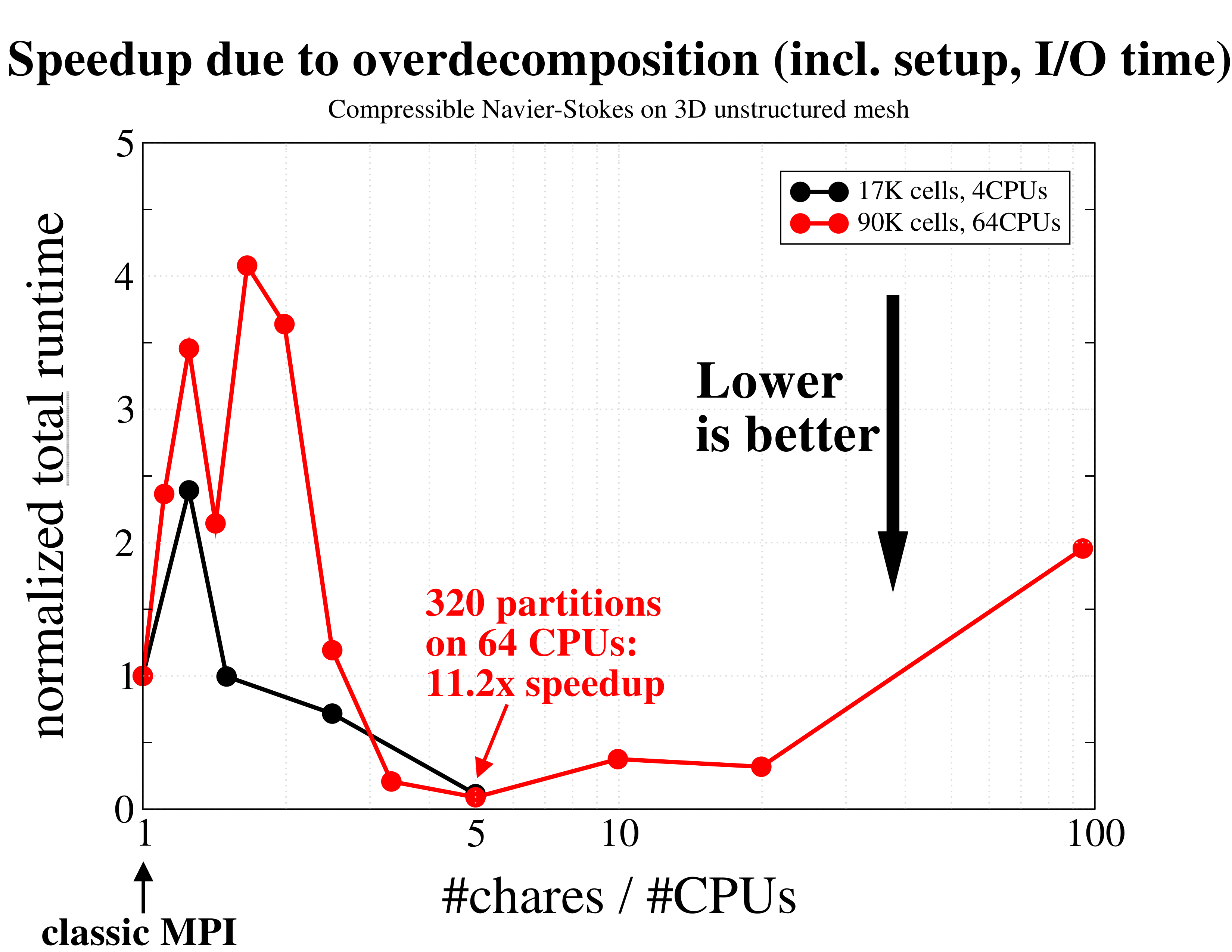Total runtime, simply measured by the Unix time utility, including setup and I/O, of integrating the coupled governing equations of mass, momentum, and energy for an ideal gas, using a continuous Galerkin finite element method. The times are normalized and compared to the leftmost (classic MPI) data. As expected, using just a few more partitions per CPU results in a performance degradation as more communication is required. However, further increasing the degree of overdecomposition to about 5 times the number of CPUs yields an excellent speedup of over 10x(!) due to better cache utilization and overlap of computation and communication.

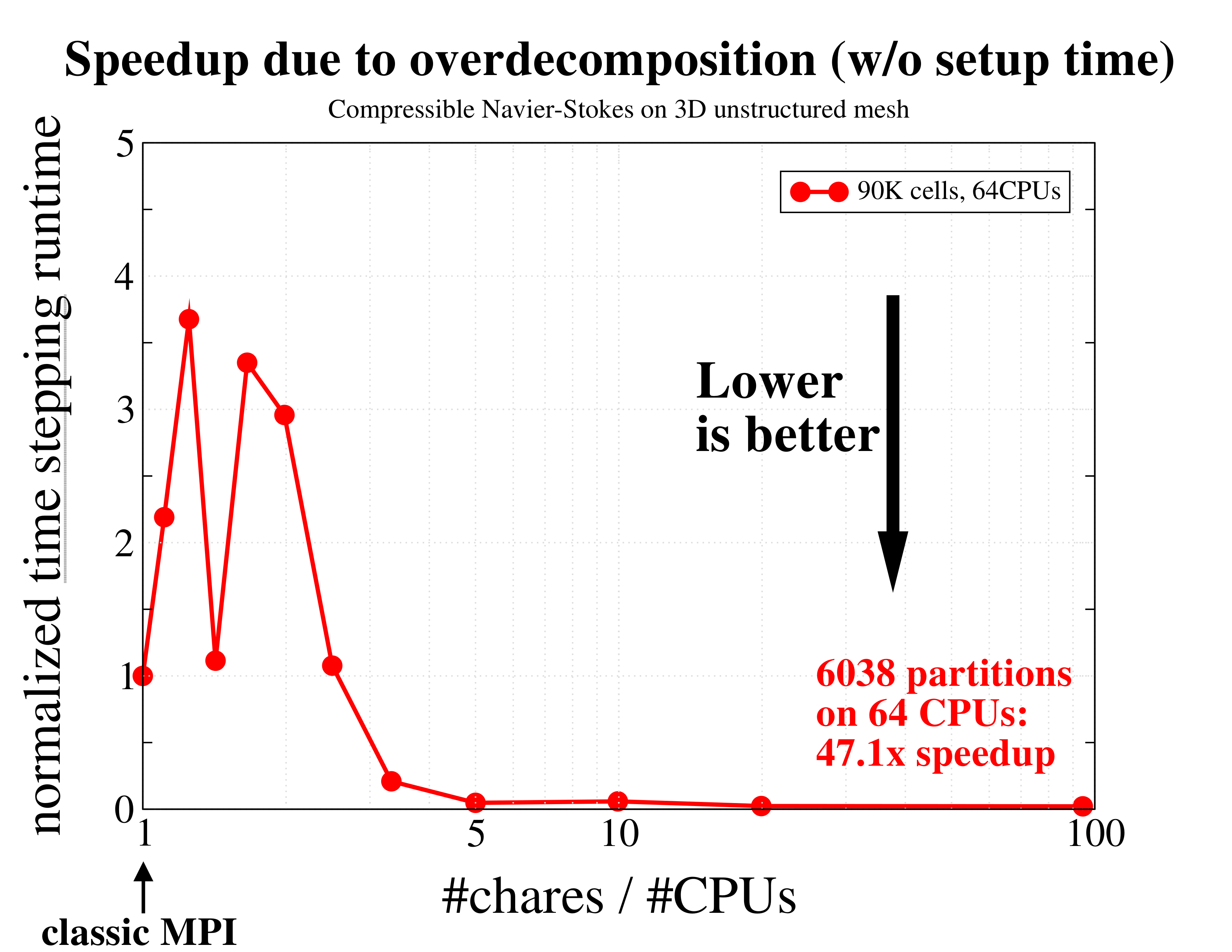This figure depicts another manifestation of the effect of overdecomposition: compared to the previous figure, here we only measured the time required to advance the equations without setup and I/O, which is usually the dominant fraction of large scientific computations. The performance gain during time stepping is even larger, reaching almost 50 times(!) compared to the original run without overdecomposition.

Load balancing

To demonstrate load balancing in parallel, we have run a Sedov problem modified to produce load imbalance. The Sedov problem is an idealized blast originating from a point, leading to a spherically spreading shock wave.

To induce load imbalance we added some extra computational load to those computational cells whose fluid density exceeds the value of 1.5. This mimics, e.g., combustion, non-trivial material equations of state, etc., and induces realistic load imbalance, characteristic of multi-physics simulations.

Spatial distributions of the extra load, corresponding to the fluid density exceeding the value 1.5, during time evolution of the Sedov solution: (left) shortly after the onset of load imbalance, (right) at end of the simulation.

One can imagine that as the computational domain decomposed into many partitions, residing on multiple compute nodes, the parallel load gets out of balance and work units must all wait for the slowest one.

Depicted below are simulation times for, running the problem using a 3 million-cell mesh on 10 computes nodes of a distributed-memory cluster with 36 CPUs/node. One can see that the density peak exceeds the value of 1.5 around the 130th time step, inducing load imbalance and this persists until the end of the simulation To balance the load we have used different strategies, available in Charm++, simply by turning on load balancing on the command line.

Grind-time during time stepping computing a Sedov problem with extra load in cells whose fluid density exceeds the threshold of 1.5, inducing load imbalance. These simulations were run on a distributed-memory cluster on 10 compute nodes, in SMP mode, using 34 worker threads + 2 communication threads per node, on a 3M-cell mesh. Load balancing was invoked at every 10th time step for all load balancers.

It is clear from the figure that multiple load balancing strategies can successfully and effectively homogenize the uneven, dynamically generated, a priori unknown computational load. The common requirement for effective load balancing is fine-grained work units, ensured by increasing the degree of overdecomposition (virtualization) from 1 to 100x, which yields 100x the mesh partitions compared to the number of CPUs the problem is running on. As expected, increasing the number of partitions beyond the number of CPUs has a cost due to increased communication cost, c.f., black and red lines. Overall however, load balancing yields over an order of magnitude speedup over the non-balanced case.